Observability and Detectability

• State Estimators
• Observers
  • Open Loop Observer
  • Closed Loop Observer with Output Feedback
• Observability and Detectability
• The Noise Problem

State Estimators

Previously I have discussed how state feedback can be used to stabilise a system and how to choose these parameters for the state feedback using LQR. However, in both these cases it was assumed that we could measure the full state of the system. Unfortunately, this is rarely the case in practical implementations. As such, state estimators are used to attempt to estimate the state of our system given some measurements.

A cart with a pendulum attached to it

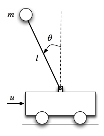
For example, consider the cart and pendulum system above and assume the input is the force on the cart. Assume that we have encoders on the wheels of the cart and the rotational point of the pendulum so that we can measure their position. Despite this, the state of the system is also dependent on the velocities of the cart and the pendulum which we are not directly measuring. In this case, we may attempt to differentiate the measured positions to determine the velocities however if the sensors are noisy then these estimates of velocity may not be accurate. We could attempt to add a low pass filter to the encoder measurements before differentiating it to try to reduce some of this noise but this will add delay to the measurements which may be unacceptable.

Observers

Open Loop Observer

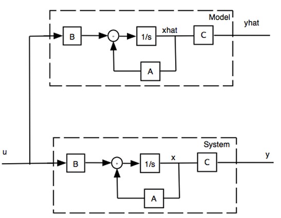
We might instead ask, is there some way that we can incorporate the knowledge about our system dynamics into the estimate for the state? To begin, we could create a simulation of the system and apply our inputs to it. This simulation would then give us both an estimate for the output $\mathbf{\hat{y}}$ and an internal estimate for the state $\mathbf{\hat{x}}$. This state estimate could then be used as the state feedback to produce appropriate inputs for the system.

A block diagram of an open loop observer

This known as an open loop observer since we just feed in the input to both systems and then rely on our model to perfectly match the real system. Firstly we can define the error to be

\[\mathbf{\tilde{x} = x - \hat{x}}\]

Then we know,

\[\begin{align*} \mathbf{\dot{x} - \dot{\hat{x}}} &= \mathbf{Ax + Bu - A\hat{x} - Bu} \\ \implies \mathbf{\tilde{\dot{x}}} &= \mathbf{A\tilde{x}} \end{align*}\]

From this we know that if our system is stable the error will converge to 0 over time but we can’t increase the speed at which it will converge. Inaccuracies in the model for our system due to linear approximations or parameterisation errors may also lead to errors in the state estimate.

Closed Loop Observer with Output Feedback

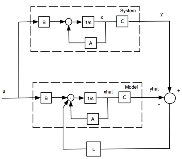
Instead, it would be better to try to incorporate the measurements from the real system to help get a better estimate of the state faster. To do this we will define the output feedback gain matrix $\mathbf{L} \in \mathbb{R}^{i \times p}$ where $i$ is the number of inputs to the system and $p$ is the number of outputs.

A closed loop observer block diagram

So now we have

\[\begin{align*} \mathbf{\dot{\hat{x}}} &= \mathbf{A\hat{x} + Bu + L(Cx - C\hat{x})} \\ \implies \mathbf{\dot{\tilde{x}}} &= \mathbf{(A - LC)\tilde{x}} \end{align*}\]

Therefore, the eigenvalues of $\mathbf{(A - LH)}$ determine how fast the error will converge and these can be controlled by choosing an appropriate $\mathbf{L}$ matrix.

Observability and Detectability

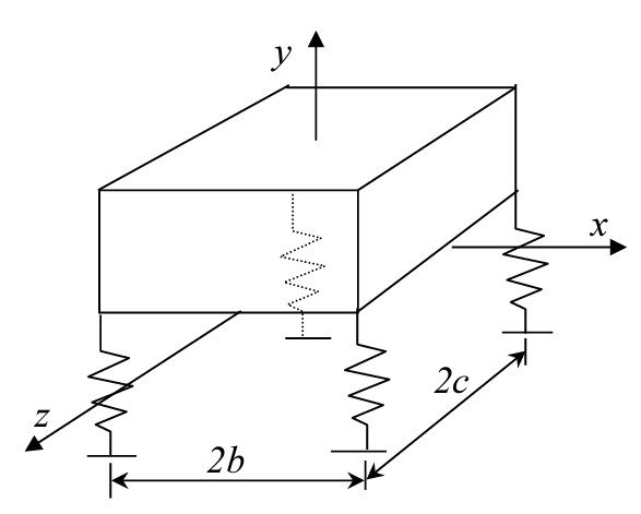
Another question it may be worth asking is can we even reconstruct the full state given our measurements? In this example, we know we could have by taking the derivatives of each of the measurements but what about a more complex system with coupled modes? For example, consider the rigid body with mounts below. This may represent a car’s suspension system.

A rigid body with mounts modelled as springs

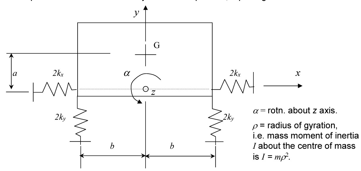A planar view of the rigid body with transverse (horizontal) springs to model the transverse stiffness of the mounts

For the planar case, do we need to measure all of $x,\, y$ and $\theta$ to estimate the full state? The answer is actually no because $\theta$ and $x$ form coupled swaying and rocking modes (try modelling this and finding the modes to check). Therefore, if we have a model of the system we could just measure one and deduce the other.

Observability and detectability are analogous to controllability and stabilisability in that they determine whether a system’s state can be fully reconstructed (for observability) or at least all of the unstable modes can be reconstructed (for detectability) from the measured outputs of the system. Just as there is a control canonical form and controllability matrix, there is also an observer canonical form (denoted with subscript o) and observability matrix (denoted $\mathcal{O}$).

\[\begin{align*} \mathbf{F_o} &= \begin{pmatrix} -a_1 & 1 & 0 & \dots & 0 \\ -a_2 & 0 & 1 & \dots & 0 \\ \vdots & \vdots & \vdots & \ddots & \vdots \\ -a_{n-1}& 0 & 0 & \dots & 1 \\ -a_n & 0 & 0 & \dots & 0 \end{pmatrix} \\ \mathbf{B_o} &= \begin{pmatrix} b_1 \\ b_2 \\ \vdots \\ b_n \end{pmatrix}, \quad \mathbf{C_o} = \begin{pmatrix} 1 & 0 & \dots & 0 \end{pmatrix} \\ \mathcal{O} &= \begin{pmatrix} \mathbf{A} \\ \mathbf{CA} \\ \vdots \\ \mathbf{CA^{n-1}} \end{pmatrix} \end{align*}\]

This is mathematically the same problem as choosing the state feedback which I showed here and so these problems are known as dual problems. Specifically, the problems are the same if you replace $\mathbf{A}$ with $\mathbf{A^T}$, $\mathbf{B}$ with $\mathbf{C^T}$ and $\mathbf{C}$ with $\mathbf{B^T}$. This can be shown quite easily since the eigenvalues (poles) of a matrix and its transpose are the same. Therefore, finding the poles of $\mathbf{A - LC}$ is the same as finding the poles of $\mathbf{(A - LC)^T = A^T - C^T L^T}$ which has the same form as the control problem $\mathbf{A - BK}$ with the above substitutions. Similarly to the control problem, we can check if a system is observable or detectable by checking the rank of $\mathcal{O}$ or using the PBH test.

Great! So if the system is observable we can choose the poles of the observer arbitrarily and make the error converge as fast as we like. What’s more, the observer is implemented in simulation so there is no physical limitation on the gain. So we should just make the gain super large so that the system converges the fastest, right? Well, not quite.

The Noise Problem

Unfortunately, in real systems there is noise. In general, we can categorise the noise as process noise, $\mathbf{w}$ which affects the state of the system and sensor noise, $\mathbf{v}$ which affects measurements of the output. Mathematically we can model these effects

\[\begin{align*} \mathbf{\dot{x}} &= \mathbf{Ax + Bu + B_n w} \\ \mathbf{y} &= \mathbf{Cx + v} \\ \implies \mathbf{\dot{\tilde{x}}} &= \mathbf{(A - LC) \tilde{x} - B_n w - Lv} \end{align*}\]

This shows that if the gain of the $\mathbf{L}$ matrix is large then the sensor noise will cause large errors. On the other hand, if $\mathbf{L}$ has small gains then the sensor noise will not impact the error too much but the response to disturbances will be slow. Therefore, there is a tradeoff. So how can we choose an optimal state feedback? Well I’m going to save that for my next post!